During my time in Europe, I was fortunate enough to travel quite extensively (an index of my travels can be found here). During my travels, I also took quite a few photos. With some time and determination, I tried to produce some figures whose content would be interesting to traveller and photographer alike. I have also included some snippets of code to help anyone should they wish to perform something similar.

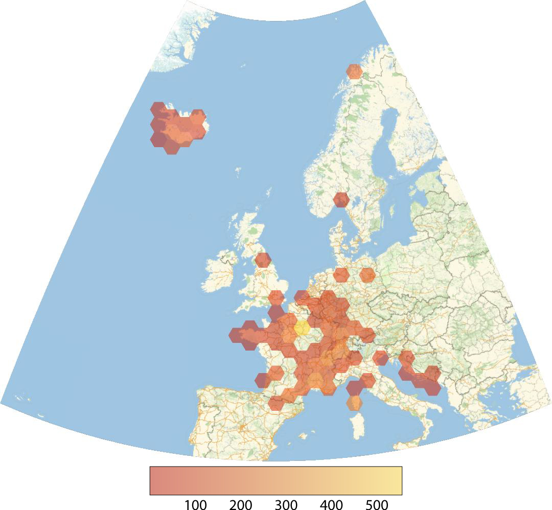
Density map of photographs taken whilst living in Europe

The above plot shows the density of photographs taken in a given region. It is clear that Paris was where much of the action happened. Given I was living there, this is unsurprising. For those with a keen eye, it is also evident that the density is elevated in the Alps, Provence, Southern Corsica and also in northern Norway.

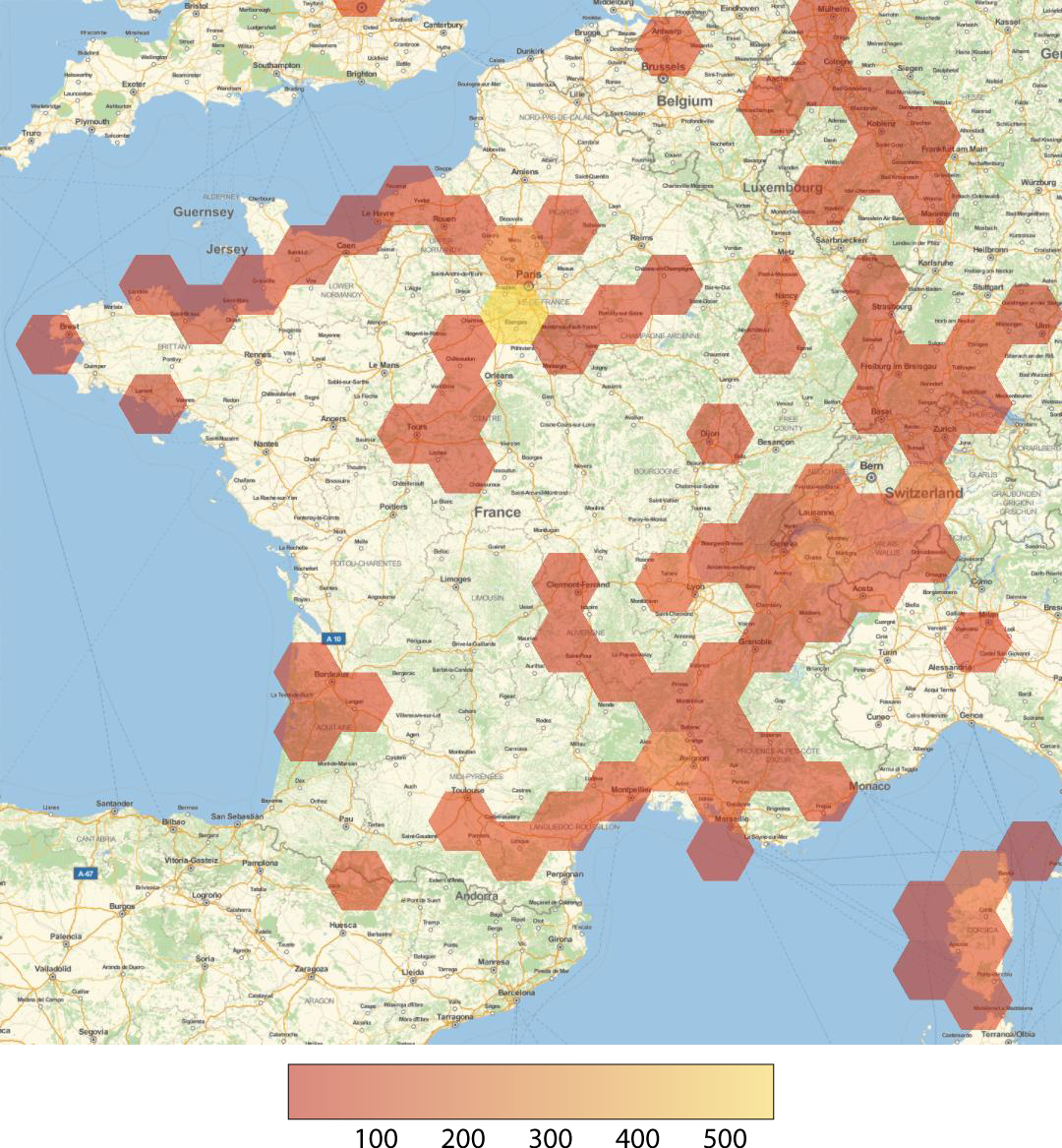
Shown on the left is the same plot, zoomed in on France, showing the regions to which I travelled and those to which I did not. Can you tell that I like mountains?

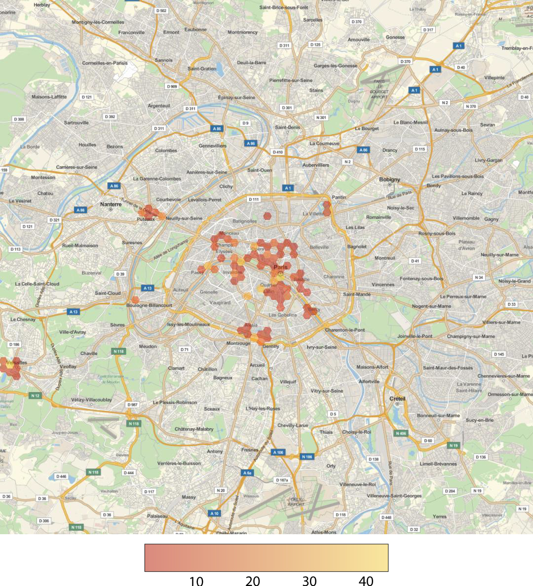
Density of photos taken in and around Paris

Paris is where many of the photos was taken, so it deserves a close-up. You can see the hot spots around the Île de la Cité and also Versailles. The oddity would be the photos taken in the south of the city, in the 14th arrondissement; however this is where I lived!

One of the cutest maps that I produced came from our trip to Iceland, where we hired a car and explored the island for two weeks. As we did not hire a four-wheeled drive vehicle, we were basically limited to excursions on and around the ring road - with the notable exception of the Vestfirðir. The map really shows where some of the amazing destinations are, with Skaftafell and Landmannalaugar particularly noticable.

The code I wrote to produce the maps takes the GPS data stored in .jpg files (or any other file format), manipulates the format of the data and ultimately exports it to be plotted. Most of the coding is done in Python, with the final plotting done in Mathematica. The GPS data had been encoded by me, using Lightroom. This is tedious, but something that I am used to doing as soon as I import my photos, along with applying keywords. Of course, if you take images with a phone or camera with GPS enabled, this step is not necessary.

Below, I will step through the code required to produce the maps, along with some bonus plots.

The following piece of code will return a dictionary of the EXIF (EXchangeable Image Format)

# get the exif info from the JPEG files
def get_exif(fn):
    ret = {}
    i = Image.open(fn)
    info = i._getexif()
    for tag, value in info.items():
        decoded = TAGS.get(tag, tag)
        ret[decoded] = value
    return ret

from which one can extract the gps coordinates:

# get the gps coordinates from the exif
def getgps(img):
    gps=None
    fulldata=get_exif(img)
    if 'GPSInfo' in fulldata:
        gps=fulldata['GPSInfo']
    return gps

# rentun the gps value in dms with "N,S,E,W"    
def interpretgpsdms(coords):
    lat = []
    long = []
    
    lat = getdms(coords[2])
    long = getdms(coords[4])
    lat.append(coords[1])
    long.append(coords[3])
    return [lat,long]

# Return decimal GPS values
def interpretgpsdec(coords):
    lat=x[0][0]+(x[0][1]+(x[0][2]/60))/60
    if x[0][3] != 'N':
        lat = 0 - lat 
    
    long=x[1][0]+(x[1][1]+(x[1][2]/60))/60
    if x[1][3] != 'E':
        long = 0 - long
    
    return [lat,long]

And finally, one can put everything together to scan a directory located in "DIR" for .JPG files

# find the images from which to extract metadata
images=[]
for file in os.listdir("DIR"):
    if file.endswith(".jpg"):
        images.append("DIR"+file)

# get the gps values for all the images
data=[]
for image in images:        
    data.append(getgps(image))

data=filter(None,data)
fdata=[i for i in data]
    
# interpret the gps values of the images    
intdata=[]
for x in fdata:
    intdata.append(interpretgpsdms(x))
    
decdata = []
for x in intdata:
    decdata.append(interpretgpsdec(x))

# write the data to a file
csvfile = "gpsoutput.csv"    
with open(csvfile,"w") as output:
    writer = csv.writer(output, lineterminator='\n')
    writer.writerows(decdata)

The output .csv was then interpreted in Mathematica using the GeoHisogram function.

file = "gpsoutput.csv";
fileloc = NotebookDirectory[] <> file;
gpsdata = Import[fileloc, "Data"];
GeoHistogram[gpsdata]

Note that by altering the function getgps, one can extract other information from the EXIF, for example:

    if 'FocalLengthIn35mmFilm' in fulldata:
        focal=int(fulldata['FocalLengthIn35mmFilm'])

Number of images taken at varying focal lengths. Inset: Zoom of the region between 10 and 60 mm

will return the focal length (in 35 mm film equivalent). This image can be seen to the right and contains a number of interesting features. Firstly, it shows that I like shooting at the wide end, with many images taken at 16 mm and 28 mm, which are the minimum focal lengths of two of my lenses, an AF-S Nikkor 16-35mm f/4G ED and an AF-S Nikkor 28-300 mm f/3.5-5.6G ED VR. There are also spikes at 35 mm and 300 mm, suggesting that I like the extremes of these lenses. The other spike is at 50 mm and is due to my fixed focal length AF-S Nikkor 500 mm F/1.4G.

Number of images taken at varying f-number

I also performed a similar analysis for the f-number, which shows that I like to shoot wide-open. Other than the peaks at 3.5 and 5.6, it is clear that 'f/9 and be there' is firmly entrenched in my style. The peak at f/16 is also quite significant, and I suppose I attribute that to those beautiful sun stars!

Number of images taken as a function of ISO

Analysing the ISO values proved much less interesting, showing that I am shooting at the lowest ISO I can get away with, which appears to be ISO-100 most of the time.

Tales of interest

Photographing Europe